Introduction

In this post, we will learn and understand why should we scale a KNN model. Prima-facie it looks like euclidean distance should not get impacted even with unscaled data i.e.

$$distance = \sqrt(X_2^2 - X_1^2) + (Y_2^2 - Y_1^2)$$

We can observe, the same feature is used in squared difference. So if Y1 is at a bigger scale so is Y2. Hence, this distance metric will remain consistent

Depicting the scaled data

The above plot is depicting two classes based on two features that are properly scaled. One of the points is highlighted in a red dotted circle. If we observe, this point very comfortably looks like a "Blue" class as almost all the neighbours are Blue.
But now try to imagine unscaled data where one of the features is large. What it means is that space will be very elongated for that axis and squizzed for the other axis.

It will mean that the distance in the smaller axis has no relevance as compared to the larger axis. The distance along the larger axis will define the total distance.

What it means for this plot is that the highlighted point has many "Orange" neighbours now since we can ignore vertical distance. These new neighbours are all the "orange points" below the highlighted point in the unscaled data. In the previous view(unscaled view) these were looking further, hence were not a Neighbour.

Let's see,

We have intentionally flattened the plot along one axis to develop better intuition. Now we can observe that the highlighted point is fairly near to the Orange" class.

Let's squeeze again,

Now, we can easily see that the highlighted point belongs to the "Orange class".

Another simple exercise

• Let's fit a KNN model on a scaled dataset and predict the class for the same data.
• Then predict the same model on the unscaled data.
• Note the point which changes their stance between the two predictions.

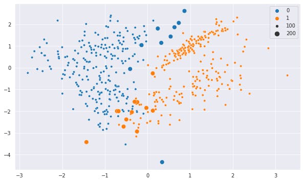
In the below plot, we highlighted the data which changed its Class with a bigger size. Hue is as per the prediction of the scaled model.

Let's see the same plot in squeezed axis and hue on prediction on unscaled data.

It is pretty evident from the above plot which data point changes its Class and why it did so. These are the points which have many data points of other class farther away on the vertical axis but very near on the horizontal axis.
With scaled data, Vertical distance lost its relevance and the Class swapped.

Code

Below is the code snippet for all the trials we did in this post.

# Create the data
import numpy as np, seaborn as sns, matplotlib.pyplot as plt
sns.set_style("darkgrid")
sns.set_context(font_scale=1.0, rc={"lines.linewidth": 2.0})

from sklearn.datasets import make_classification
x, y = make_classification(n_samples=500, n_features=2, n_classes=2, 
                           n_informative=2, n_redundant=0)

# Simple plotting the points
fig = plt.figure(figsize=(10,6))
sns.scatterplot(x = x[:,0], y = x[:,1], hue=y)

# Flattened the axis and Unscaled the data
fig = plt.figure(figsize=(20,1))
sns.scatterplot(x = x[:,0]*100, y = x[:,1], hue = y)

# Further Flattened the axis and Unscaled the data
fig = plt.figure(figsize=(20,0.5))
sns.scatterplot(x = x[:,0]*100, y = x[:,1], hue = y)

# Created the Model and fit the data
from sklearn.neighbors import KNeighborsClassifier
model = KNeighborsClassifier(n_neighbors=3)
y_pred = model.fit(x, y).predict(x)
x[:,0] = x[:,0]*200
y_pred_unscaled = model.fit(x, y).predict(x)
diff = y_pred!=y_pred_unscaled

# Plot for scaled prediction and highlighting the diff data points
fig = plt.figure(figsize=(10,6))
sns.scatterplot(x = x[:,0]/200, y = x[:,1], hue=y_pred, size=(diff+1)*100)

# Plot for unscaled/Elongated axis, prediction and highlighting the diff data points
fig = plt.figure(figsize=(20,3))
fig.gca().set_ylim(-10,10)
sns.scatterplot(x = x[:,0], y = x[:,1], hue=y_pred_unscaled, size=(diff+1)*100)

Code-explanation
^{All other parts of the code is quite trivial and self-explanatory.}

Conclusion and Summary

So, what is meant is that if we use unscaled data, the distance along the Feature having a smaller value will lose its relevance. The issue will impact the boundary points and it will become more severe if the two Features differ on a large scale.
So, it's better to scale even though it is not needed because it will not create any problem if done unnecessarily.
Similar logic can be applied to Clustering using KMeans as that algorithm is also based on the same approach.