Introduction

In this blog post, we will learn how to catch the Outliers Or Anamolous data points. Don't worry about the terminology, we will start with the meaning first.

In the process, we will look into 4 key algorithms for the purpose and also understand the working of these algorithms. We will also learn to program aa simple Anomaly detector using these algorithms. You may also use these approaches in Exploratory Data Analysis steps to figure out the Outliers.

We will Learn,

• Clarifying the taxonomies around Anomaly detection
• Understanding and applying IsolationForest
• Understanding and applying GaussianMixtureModel
• Understanding and applying LocalOutlierFactor
• Using the reconstruction error of PCA

Understanding the Taxonomy

Let's start with the definition of important terminologies.

1. Anomaly/Outlier - We assume a certain pattern in our datasets and any data points which is far away from the pattern are considered as Anomaly. Or we can say, farther the point more is the chance of it to be an Anomaly. The normal data points are called Inliers. The task is to figure out an approach to define distance and a threshold to define the boundary for Inliers(Normal) vs Outlier(Anomalous)
2. Novelty detection - Problem and underlying idea remain the same but the approach to apply the solution changes. We take a semi-unsupervised Machine learning approach here. We use only the Inliers datasets and train the Model. Then we can use a few of the labels to decide a Threshold of distance to identify the Outlier. Treat any new dataset which is beyond the Threshold as New i.e. Novel. In the case of Anomaly detection, we can take a Supervise approach and utilizing the Outlier to decide the decision boundary between the Outlier and Inliers. but in this case, we have to figure out a Threshold-based on expert-judgment or few data points
3. Class Imbalance - Class imbalance is when the dataset is not evenly balanced between multiple classes. This problem can become a special case of Anomaly detection when the percentage of minority class is very low. We will not discuss Class-Imbalance in this post.

   ^{Semi-supervised Learning - This is an approach where we utilize the available Label for some datasets to figure out the labels of other datasets using Unsupervised learning and then apply Supervised Learning on the whole dataset. We have used this term for a little different approach where we will use the Label to figure out the Threshold for Normal-Anomaly boundary}

Class boundary and general approach

Let's try to see how Normal-Outliers will look in different scenarios and what all approaches we may take to figure out the difference.

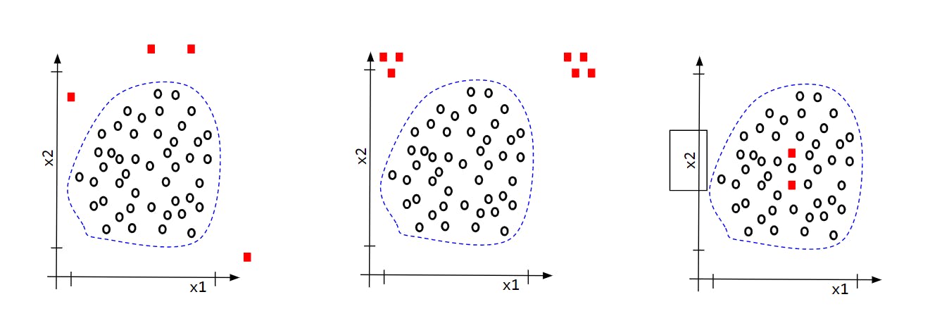
We will try to figure out the Outliers of Scenario-I and II. For Scenario-III we will need a close analysis of the two data points and need to come up with a new Feature for the Model which can distinguish between the Normal and Anomaly

Possible approaches

• Get the distance of all the points from all other points. The Outliers will have a higher average distance
• Neighbor of the neighbour of an Outlier is the Outlier itself
• If we build a Clustering model which assign the probability of belongingness to the Cluster to each point, then Outliers will have a smaller probability
• If we build a DecisionTree to segregate each data points, chances are high that an Outlier will be segregated to a Leaf very early in the Tree

Our Dataset and approach

We will use the classic KDD Cup ‘99 dataset. The KDD Cup ‘99 dataset was created by processing the tcpdump portions of the 1998 DARPA Intrusion Detection System (IDS) Evaluation dataset, created by MIT Lincoln Lab. We will use the "http structure" subset of the dataset with 3 Features

In our training, we will only use the Normal data points and build a Novelty detector. We will use the Outlier data point as new data points in the testing stage.

Let's see the Code

import numpy as np, pandas as pd, matplotlib.pyplot as plt, seaborn as sns
from sklearn.datasets import fetch_kddcup99

dataset = fetch_kddcup99(subset='http', shuffle=True,  return_X_y=False)
x, y = pd.DataFrame(dataset.data),pd.DataFrame(dataset.target)
# Let's keep only normal and back.
x = x.loc[y.isin([b'normal.',b'back.']).values]  #1
y = y.loc[y.isin([b'normal.',b'back.']).values]

x_train = x.loc[y==0,:] #2
x_test_outlier = x.loc[y==1,:] #3

from sklearn.model_selection import train_test_split
x_train,x_test_normal = train_test_split(x_train,test_size=2500) #4

Code-explanation
^{#1 - Filter the dataset to keep only one type of Outliers. Full dataset has multiple types
#2, #3 - Filter Inliers as x_train and Outliers as x_test(Positive)
#4 - Filter another dataset out of Inliers as a separate x_test(Negative)
All other parts of the code is quite trivial and self-explanatory.}

We will build multiple Models for the dataset. Let's start with Gaussian Mixture Model.

Model - I - Gaussian Mixture Model

How it works

GMM model learns to find a weighted mixture of multiple Gaussian distributions across the dataset. Hence, we get a probability for each data point for its belongingness for each individual Gaussian fit. Check the depiction below

We can observe the contours of the mixture of two Gaussian. The probability decreases as the points move farther away from the mean. So the outlier points will have a small probability for both the Gaussian components.

Let's see the Code

from sklearn.mixture import GaussianMixture

aic = []
for n in range(1,10):
    gm = GaussianMixture(n_components=n, random_state=0,n_init=10).fit(x_train)
    aic.append(gm.aic(x_train))

sns.lineplot(x=np.arange(1,10),y=aic) # To identity the best n_components

Code-explanation
^{n_components is the number of Gaussians we want to mix in the Model. Just like we use silhouette_score for KMeans we use the Akaike information criterion[ AIC ] for GMM. In this case we got best n_components=2}

gm = GaussianMixture(n_components=2, random_state=0,n_init=10).fit(x_train)

proba_train = gm.predict_proba(x_train) #1
threshold = np.percentile(proba_train, 2.5, axis=0) #2

score_test_normal = gm.predict_proba(x_test_normal)
x_test_normal.loc[score_test_normal < threshold] #3

score_test_outlier = gm.predict_proba(x_test_outlier)
x_test_outlier[score_test_outlier < threshold] #4

Code-explanation
^{#1 - Calculate the probability for each data points for each Gaussian component
#2 - Calculate a Threshold of probability considering the 2.5 percentile as Threshold. This is just a common guess here. Should be driven by case
#3 - Filter the records which are having a lesser probability than the Threshold from x_test_normal . This will be our "False Positive"
#4 - Do the same for x_test_outlier . This will be our "True Positive"}

Result
^{Outliers - All 2203 out of 2203 identified
Normal - 135 out of 2500 incorrectly identified}

Conclusion and way forward

Now we understand different taxonomy around Outliers and Novelty detection. We also learnt one of the approaches to figure out the Outliers. In the next post [Link ], we will continue with the remaining models i.e. Isolation Forest, LocalOutlierFactor and PCA. See you there.