Introduction

Hello AI Enthusiasts, with this post we will start a series of posts on Natural Language Processing(NLP). We assume you have a basic understanding of ML and DL around tabular data. You can treat this series as a smooth transition from your current knowledge into the NLP space.
We can't covert every part and bit of such a huge space, so we will summarize that(Not covered topics) too at the end. We will also learn the related code. In the journey, we will try to answer many of the confusing questions and concepts.
Below is a depiction of our intention.

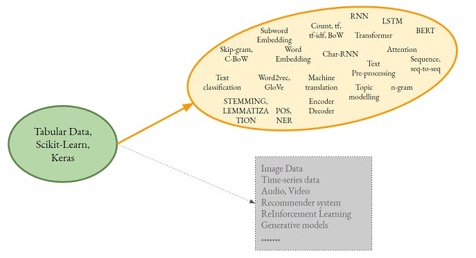As you may observe, we will cover a broad range of topics. The focus is on understanding the Algorithm and Feature engineering techniques. We have escaped the NLU (Natural Language Understanding) zone which makes the foundation of Chatbots, conversational AI. So. let's start the journey.

Text Preprocessing

The first thing that we will analyse is the structural difference in the dataset as compared to a Tabular dataset.

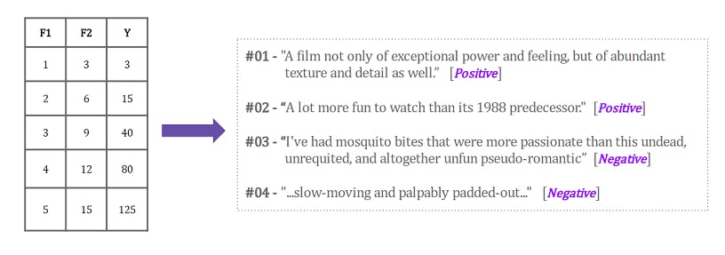
As shown in the above depiction, features were defined and very well organized in the case of a Tabular dataset. But in the case of a Text dataset,

• Features are not define
• Hence, not segregated
• Datapoint has different lengths
• Dataset is 100% Nominal(Obviously)

Preprocessing is all about handling the above scenario. Text data preprocessing requires more effort as compared to the Tabular counterpart. One aspect that we didn't list is the cleansing of text. We will use a fairly clean dataset, so we will skip this part. We will use the IMDB movie review dataset.

Let's check the different terms and steps -

1. Tokenization - Tokenization is the step where each text sequence is split into a list of tokens. A token is a basic unit in the text. In our current case, it is a Word e.g. "exceptional ". With this step, we got our Features. But it is still a bit far from use.

2. Vocabulary(Bag-Of-Words) - This is the key step in finalizing our Features from the sentences. We build a vocabulary list for all the unique words(Tokens) available in our dataset. This is also known as Bag-Of-Words. This is the simplest form of words i.e. 1-gram(more on it later). It must be noted that the Documents are described by word occurrences while completely ignoring the relative position information of the words in the document.
   What if a word is new and came only in the test dataset. This is called Out-Of-Vocabulary. It is handled by keeping placeholder word. All new words will be mapped to that word. Definitely, it will not help much in the prediction. There are some other flavours for this. We will also learn that later.

3. One-Hot-Encoding - With this last step we are ready to create our Features. We will have one dimension for each unique word and simply mark the respective feature value "one" if it is present in the document. In case the word is absent, we will mark it as "zero". This was a simple multi-label One-Hot encoding

4. Term-frequency(tf)- With a plane Multi-label OHE we are losing the information of reoccurrence of a word. It may not impact the Positive-Negative class separation but it will bring all the document of the same class nearby-by i.e. not adding much value in term of class-probability. With term-frequency, we put the count of each Token as a feature value instead of just 0/1.

5. Normalized Term-frequency - Different document can be of different length. One of the many implications of this is that a particular document may get a bigger frequency of a Token only because its length is more than the other e.g. a 10 Token document has "Happy" two times while a 5 Token document as it only once. So, we simply divide the term-frequency by the length of the document.

6. Term-frequency Inverse Document Frequency(tf-idf) - Imagine a word that is present in almost every document i.e. "The". Although this will not impact the Classification boundary but it will add an unnecessary Feature. So, we simply divide each Token by its document-frequency i.e. the number of document it is present in. This new entity is tf-idf. It has more significance in the Search algorithms i.e. Google etc. not a lot here since we can remove such redundant token with other techniques too.

7. Word-embedding - This is a broad topic in itself. We will have a dedicated post on this.
   Check this depiction for an overall summary.

^{Few things we didn't talk about but we will use them implicitly e.g case normalization(all token are in small case).
Similarly, Lemmatization is the task of determining that two words have the same root, despite their surface differences e.g. play, playing. There are many dedicated algorithms for this. We will no do this in this post and rely upon our dataset.
Another one is Stop-words which those words that are very common in all the documents and have very little useful information that can be used to distinguish between different classes of documents. Examples of stop-words are is, and, has, the, like
_{May go through this beautiful book Speech and Language Processing (3rd ed. draft) Dan Jurafsky and James H. Martin to dive deeper.}}

Let's move to the Code

We are done pretty well with the terminologies. Now let's list the steps and start coding them.

1. Load the documents
   We will not do any cleaning activity as we will use a standard dataset from Keras.
2. Create features based on OHE, Term-frequency
3. Reduce the dimension
   This is a point we didn't discuss in the last section. If we will simply keep all the words in our vocabulary we will end with way too many Dimensions. We can skip words by removing stop-words Or keeping only top K features based on tf-idf.
4. Train and test with a Model

from tensorflow import keras
import numpy as np

num_words=1000; maxlen=300 ; skip_top=100

(x_train, y_train), (x_test, y_test) = keras.datasets.imdb.load_data(num_words=num_words, maxlen=maxlen, skip_top=skip_top) #1

type(x_train)
max_doc_len = max(np.vectorize(lambda x : len(x))(x_train)) # This is the word count for the longest document

Code-explanation
^{#1 - A available function in in keras.datasets. It return the numpy array of the dataset
num_words - Words are ranked by how often they occur (in the training set) and only the num_words most frequent words are kept. Any less frequent word will appear as oov_char value in the sequence data. If None, all words are kept. Defaults to None, so all words are kept.
skip_top - skip the top N most frequently occurring words (which may not be informative). These words will appear as oov_char value in the dataset. Defaults to 0, so no words are skipped.
maxlen - Maximum sequence length. Any longer sequence will be truncated. Defaults to None, which means no truncation.}

This was the data load part. You right have noticed that we have controlled irrelevant words i.e. Stop words, Token count i.e. Feature Dimension using the 3 parameters that are listed above. The value of skip_top must be based on exploring the dataset but we have picked a guessed number.

Let's create a Multi-labelled OHE for the train and test dataset and fit an SVM model.

x_train_ohe = np.zeros((len(x_train), max_doc_len))
for i,documents in enumerate(x_train):
    for word in documents:
        x_train_ohe[i,word]=1

x_test_ohe = np.zeros((len(x_test), max_doc_len))
for i,documents in enumerate(x_test):
    for word in documents:
        x_test_ohe[i,word]=1

Code-explanation
^{We simply looped over each token and assign a 1 to the respective Index. All the other indexes will remain 0}

from sklearn.svm import SVC
model = SVC()

sample = np.random.randint(0, len(x_train), size=(5000))
model.fit(x_train_ohe[sample],y_train[sample])

model.score(x_test_ohe, y_test)

Result
^{Accuracy - 0.8502827763496144}

We used only the 5000 documents out of the 25K and we got almost 85% accuracy. The reason for this is that the Classification boundary is dependent on only a few keywords for the positive and negative sentiment.

Below is the code snippet on how to get the different statistical format using scikit-learn that we discussed in the previous section.

x_train_str  = np.vectorize(lambda x : ' '.join([str(elem) for elem in x]))(x_train) #1

# Term Frequency
from sklearn.feature_extraction.text import CountVectorizer
vectorizer = CountVectorizer()
x_train_count = vectorizer.fit_transform(x_train_str)

# Term frequency - Inverse Document Frequency
from sklearn.feature_extraction.text import TfidfVectorizer
tfid = TfidfVectorizer()
x_train_tfid = tfid.fit_transform(x_train_str)

Code-explanation
^{#1 - In this line we have convert the list object into String. This is the requirement of scikit-learn.
Rest of the code is self-explanatory. You may also achieve the same by a custom code i.e. using NumPy only as the steps are quite simple and trivial}

Conclusion

With the last snippet, we completed this post explaining and end-to-end concept to code journey to build a Sentiment analyzer based on IMDB Movie review dataset.
You may try -

• Smaller document length and Training size
• Apply Naive Bayes algorithm instead of SVM

We treated all the individual token as independent i.e. not accounted for their proximity Or their consecutiveness. For example, "very kool" would have lost its extra sense of emphasis on positiveness.
In the next part of this series, we will treat the reviews as a sequence i.e. will try to account for the significance of its Token's order.