Introduction

Deep Neural Network has always been a Black Box and it is still so but there are many good techniques that can help us to gain some insights about the black box.

In this 4-blog series, we will understand and code these techniques on Image data i.e. CNN. In doing so, we will go through multiple approaches.

This is Part-III of the series. In this post, we will learn to get the Class Activation Map for a CNN even when it has multiple Fully-Connected-Layers. This was one of the challenges with CAM [Read Part-II here and Part-I here ]

This approach will require a little understanding of TensorFlow GradientTape.

Gradient in a Typical CNN

In the CAM approach, we calculated the heatmap using the below formula $$CAM = \Sigma(w_i * FM_i)$$

^{w_i is the weight of the GAP Layer of i_th Feature map of the last Layer connecting to the Softmax}

Grad Cam is exactly based on the same approach, the only thing that changes is to think of an alternate entity instead of the weight which will allow the Model to have any number of FC layers after the Conv. layer.

Below is the depiction of the above idea i.e. a typical convolutional Network. Let's try to understand the idea.

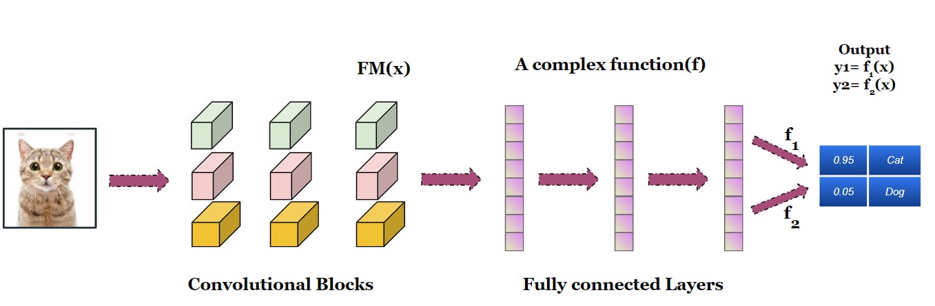
^{Note - The last Feature map are the Features for the FC Layers and we can assume the FC layer as a complex function over these Features. After the last FC layer, two different sets of weights are connected to the two output neurons, so the final function is different for different output classes i.e. f1 and f2}

Our goal is to get the impact of the last convolutional layer on the outputs. Since the outputs are a function of FM(x), the derivative of the outputs class w.r.t to the FM will directly represent how the output class will change with a small change in the FM

So, if we compare to the CAM approach, the multiplier weights are replaced by the derivative and to get the derivative we don't need a constraint on the Architecture. It can be calculated for any number of FC layers.

Steps

We will follow these steps -

1. Fit a Pre-trained model on the Cats-Dogs dataset
2. Get the Class's partial derivative w.r.t the last convolution layer's output
3. Calculated the mean of the derivative for each FM
4. Calculate the weighted result of all the FM and the Derivative i.e. Grad-CAM
5. Resize the CAM and superimpose on the original image

^{Note - As mentioned earlier, every feature map will be connected to two output Neurons with two different sets of weights, so we have to use the Derivative for that particular Class w.r.t the FM}

The Code

Define and trained a pre-trained model [ VGG16 here]

# Case - II - Train Classification layers 
import tensorflow as tf
from tensorflow import keras
from keras.applications.vgg16 import VGG16

model = VGG16(weights='imagenet')

^{Note - Model is loaded as it is i.e. we included the Top FC Layers}

In the below snippet, we calculated the Gradient of the last

# Get the gradient of the max class w.r.t the output of the conv.(last) layer
conv_layer = model.get_layer("block5_conv3")
joint_model = keras.Model([model.inputs], [conv_layer.output, model.output])

with tf.GradientTape() as gtape:
        conv_output, predictions = joint_model(img)
    y_pred = predictions[:, np.argmax(predictions[0])]

grads = gtape.gradient(y_pred, conv_output)
print(grads.shape)

^{Note - This is a typical way to get the Gradient for any Node w.r.t. any parameter list. If you want to understand the concept, check this Blog [ Link ]. For now, you may assume that grads have got the Gradients of the last convolution Layer}

In this code snippet, we calculated the weighted sum(Grad-CAM) of all the FM. Then we resize the CAM and apply a colour-map.

grads = tf.reduce_mean(grads, axis=(0,1,2))      #1
grad_cam = tf.math.multiply(conv_output,grads)    #2
grad_cam = tf.reduce_mean(grad_cam, axis=-1)[0]      #3

# Upsample (resize) it to the size of the image i.e. 224x224
import cv2
grad_cam = cv2.normalize(grad_cam, None, alpha = 0, beta = 255, norm_type = cv2.NORM_MINMAX, dtype = cv2.CV_8UC3)
grad_cam = cv2.resize(grad_cam, None, fx=224/14, fy=224/14, interpolation = cv2.INTER_CUBIC)
grad_cam = cv2.applyColorMap(grad_cam, cv2.COLORMAP_JET)[:,:,::-1]  # This slicing is to swap R,B channel to align cv2 with Matplotlib

Code-explanation
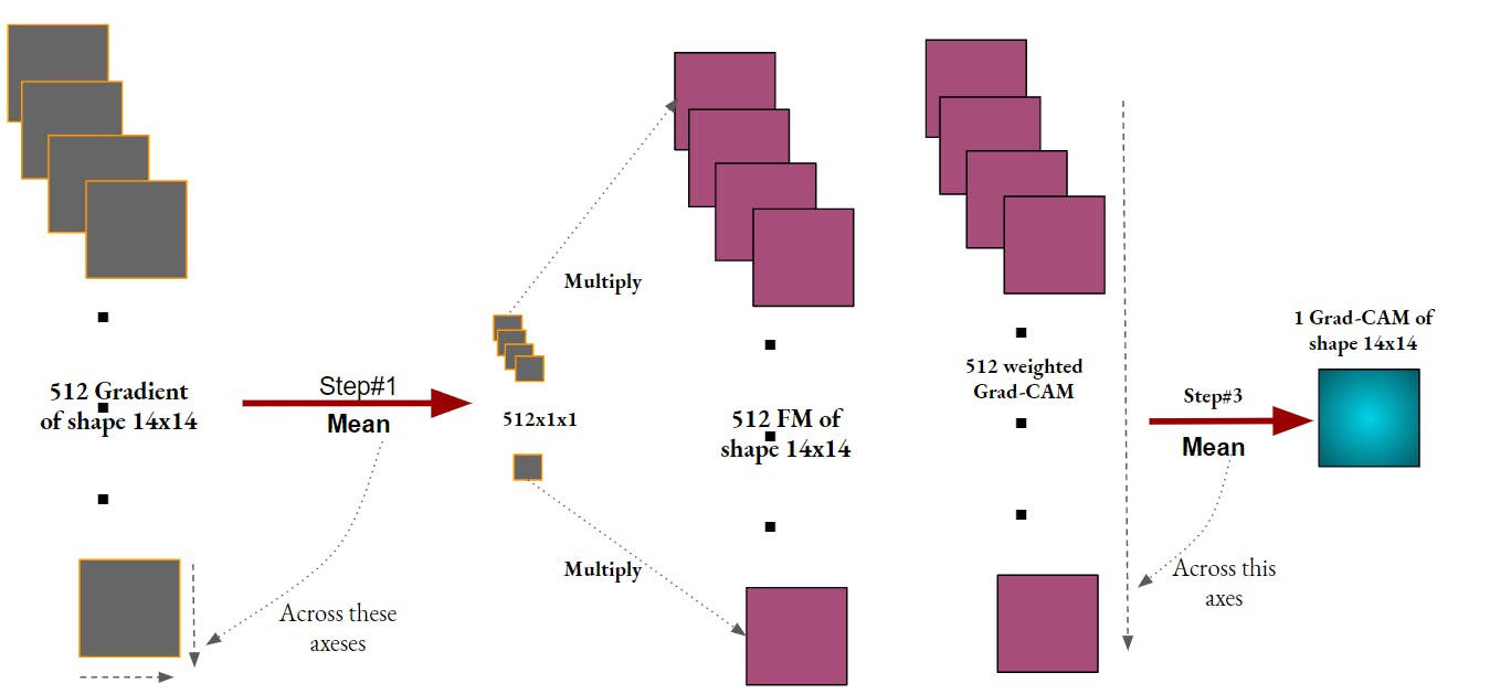
^{#1 - Calculated the mean value of each Gradient (Gradient shape is 1x14x14x512). For ImageNet it was 7x7x2048
#2, #3 - Multiplied the Grad-cam with the FM and calculated the mean across all the weighted FM}

The above operation has been depicted below Image,

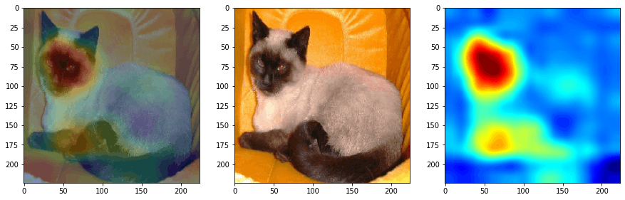
In the below snippet, we have simply Superimpose the Grad-CAM to the original image using OpenCV functions.

img = image.load_img(img_path, target_size=(224, 224)) 
img = image.img_to_array(img)
img = cv2.normalize(img, None, alpha = 0, beta = 255, norm_type = cv2.NORM_MINMAX, dtype = cv2.CV_8UC3)
superimposed_img = cv2.addWeighted(img, 0.5, grad_cam, 0.25,0)

_, ax = plt.subplots(1,3,figsize=(15,5))

ax[0].imshow(superimposed_img, cmap='jet')
ax[1].imshow(img, cmap='jet')
ax[2].imshow(grad_cam, cmap='jet')

Code-output

Summary and conclusion

This approach solved the problem created by the CAM approach i.e. we can have any number of FC layers

This can also be extended to define a bounding box across the image using a relevant thresholding approach. In the paper, there are additional use cases by blending Grad-CAM with few other known approaches. Check the paper here Link

On the down-side,

1. Though not very severe but still, it requires an extra pass of the Image through the Network
2. It is still based on upsampling the CAM so the resolution is not very high. But this issue has been solved in the paper with an improved approach

With this post,

• we are fully equipped with all the techniques required to look inside a CNN and also understand the evolution over time.
• We also understand the working of Tensorflow GradientTape

In the next part of this series, we will learn to visualize the weights and FM of convolutional layers. This will help more in understanding how the model is learning in the training.