Introduction

Deep Neural Network has always been a Black Box and it is still so but there are many good techniques that can help us to gain some insights about the black box.

In this 4-blog series, we will understand and code these techniques on Image data i.e. CNN. In doing so, we will go through multiple approaches.

This is Part-II of the series. In this post, we will visualize the image to find out the most important pixels using a technique called Class Activation Map as described in this Paper. This is too a straightforward technique, but everything is complex unless it is made simple, so all the credits to the Researchers.

Class Activation Map

Let's assume a CNN model with Conv. layers connected to a single fully connected layer via. a Global Average Pool layer. This is a very common CNN Architecture.

So, the image will be scanned with all the convolution Layer and the last Layer will have the key Features in the form of multiple Feature maps. Then using these feature maps the Fully connected layer will decide what the Category is e.g. Cat/Dog.

What it means is that the combined effect of the Feature map and the respective weight of the fully connected layer is the value that the model has for every image.

So, if we create a weighted sum of the weight and the Feature maps, it should represent the effective spatial importance (More on it later) for the image. This will represent the Class Activation Map of that Class (use weights that are connected to the particular Class Neuron of the Softmax).

Then the task that remains is to resize this map to the size of the image.

Below is the depiction of the above idea [Image is taken directly from the paper - Arxiv link]

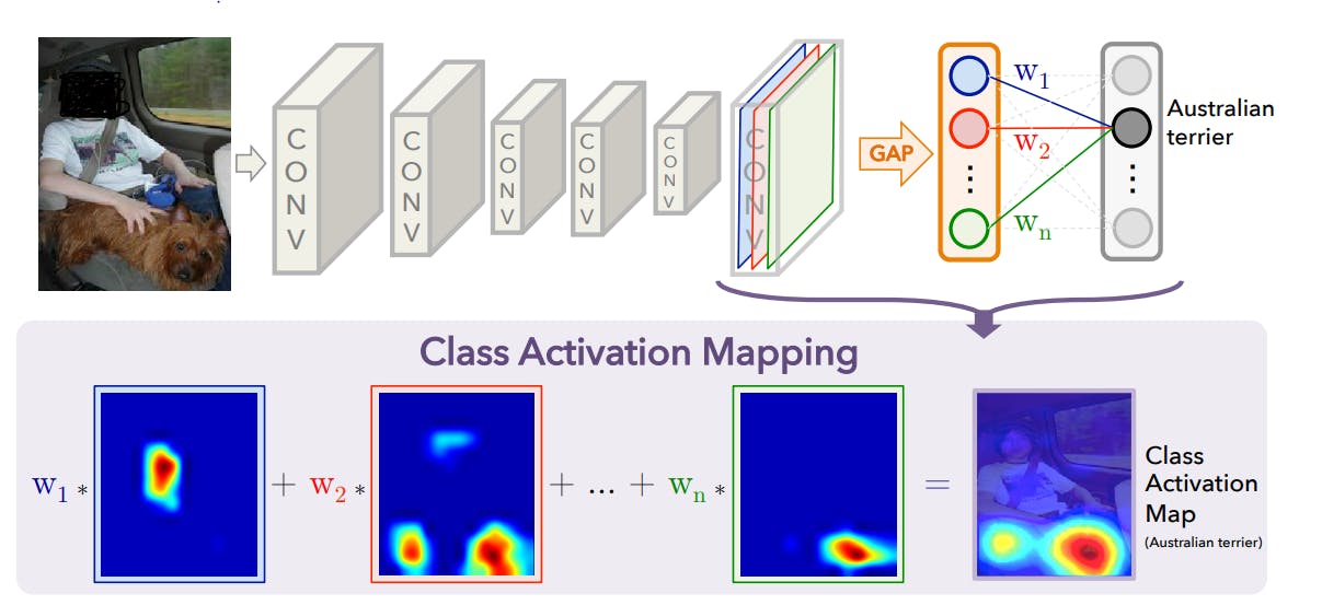
^{The Global Average Pool layer is the direct representation of the last Feature map and the weight connecting the Global Average Pool to the Softmax is the weight can be considered equivalent to a weight that is directly mapped from the FM to the Softmax}

Steps

We will follow these steps

1. Fit a Pre-trained model on the Cats-Dogs dataset
2. Get the last convolution layer's output for the Original Image
3. Get the respective weight of the feature map(FM) connecting to the Softmax
4. Calculate the weighted result of all the FM which is the Class Activation Map(CAM)
5. Resize the CAM and superimpose on the original image

   ^{Note - As mentioned earlier, every feature map will be connected to two output Neurons with two weight, so we have to use the weight for that particular Class which was predicted by the Model}

The Code

Define and trained a pre-trained model [ ResNet50 here]

import tensorflow as tf
from tensorflow import keras
from keras.applications.resnet50 import ResNet50

base_model = ResNet50(weights='imagenet', include_top=False)

model = keras.Sequential()
model.add(base_model)
model.add(keras.layers.GlobalAveragePooling2D())

model.add(keras.layers.Dense(2, activation="softmax"))

#Freeze the layers of Pre-trained models
for layer in base_model.layers:
    layer.trainable = False

optimizer = keras.optimizers.Adam(lr=0.02)
model.compile(loss="binary_crossentropy", optimizer=optimizer, metrics=["accuracy"])

#No need to train for a very long time
history = model.fit(traindata, epochs=1, validation_data=testdata)

In the below snippet, picked a random image from the folder and predict its output with an Intermediate model to get the Feature maps of the last convolution layer

img_path = '/content/train/' + str(img_list[np.random.randint(0,len(img_list))])
img = image.load_img(img_path, target_size=(224, 224)) 
img = image.img_to_array(img)
y_class = img_path.split(sep="/")[-1][:3]
img = np.expand_dims(img, axis=0)
img = preprocess_input(img)       #1

# Create a model with Conv block (only)
model_b = keras.Sequential()
model_b.add(base_model)

op = model_b.predict(img)[0] # This is 2048 FM of size 7x7

# Weights from the lasy Layer [ This is from original Model]
weights = model.get_weights()[-2]   #2
weights.shape

Code-explanation
^{#1 - This is the preprocess function of the ResNet model [Keras version]
#2 - Get the Weights(not bias) from the last layer. The index is to fetch that. [-1] will fetch the Biases}

In this code snippet, we calculated the weighted sum(CAM) of all the FM. Then we resize the CAM and apply a colour-map.

# Weights will depend on the actual class of the Image
if y_class=='cat':
    cam = op*weights[:,0].reshape(1,1,-1)
else:
    cam = op*weights[:,1].reshape(1,1,-1)

cam = cam.sum(axis=-1)

# Upsample (resize) it to the size of the image i.e. 224x224 [ResNet]
import cv2
cam = cv2.normalize(cam, None, alpha = 0, beta = 255, norm_type = cv2.NORM_MINMAX, dtype = cv2.CV_8UC3)
cam = cv2.resize(cam, None, fx=224/7, fy=224/7, interpolation = cv2.INTER_CUBIC)
cam = cv2.applyColorMap(cam, cv2.COLORMAP_JET)[:,:,::-1]  # This slicing is to swap R,B channel to align cv2 with Matplotlib

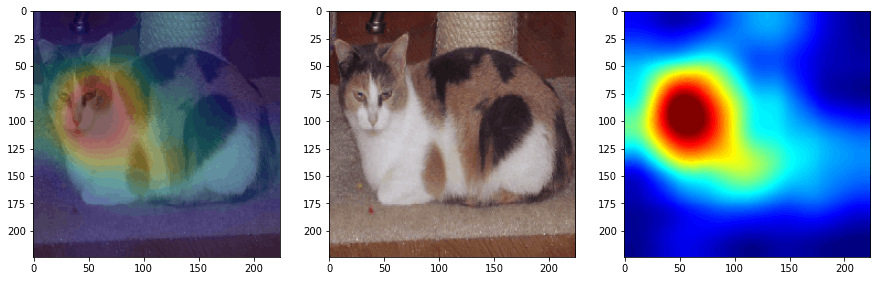
In the below snippet, we have simply Superimpose the CAM to the original image using OpenCV functions.

# Load the same image again
img = image.load_img(img_path, target_size=(224, 224)) 
img = image.img_to_array(img)
img = cv2.normalize(img, None, alpha = 0, beta = 255, norm_type = cv2.NORM_MINMAX, dtype = cv2.CV_8UC3)
superimposed_img = cv2.addWeighted(img, 0.5, cam, 0.25,0)

# Displaying with Matplotlib
_, ax = plt.subplots(1,3,figsize=(15,5))

ax[0].imshow(superimposed_img, cmap='jet')
ax[1].imshow(img, cmap='jet')
ax[2].imshow(cam, cmap='jet')

Code-output

Summary and conclusion

This approach was quite simple and also no special computation was required like the occlusion method.

We can also extend this to define an abounding box across the image using a relevant thresholding approach. Though the Box would be more on the CAM rather than the full object.

On the down-side,

1. CAM can not be applied to networks that use multiple fully-connected layers before the output layer, so fully-connected layers are replaced with convolutional ones and the network is re-trained. It expects a single fully connected layer post the global average pol layer.
2. It is still based on upsampling the CAM so the resolution is not very high

So, we need an approach that doesn't need these restrictions. That is where we apply the concept of Grad-CAM Arxiv link

We will learn this technique in the next part of this blog series. Check it Here Link