Introduction

Deep Neural Network has always been a Black Box and it is still so but there are many useful techniques that can help us to gain relevant insights about the black box.

In this 4-blog series, we will understand and code these techniques on Image data i.e. CNN. In doing so, we will go through multiple approaches

Ways using which we may look into CNN,

• Looking at the Filters
• Looking at the Convolution feature map
• Class activation map

This is a family of techniques. The key goal of each is to find out which part of the image is more responsible for the output. Definitely, another added goal is to do this efficiently otherwise this is an easy task.

Class Activation map (heat map)
^{A heatmap across the image's pixels according to the importance of the pixel for a particular output Image courtesy - Matthew D. Zeiler, Arxiv link}

Key approaches for getting the Class Activation map (heat map) are

• Occluding parts of the image as described in this paper Arxiv link
• Simple CAM as described in this paper Arxiv link
• Grad-CAM as described in this paper Arxiv link

In this post, we will look into the first approach. This is very simple and will give us the optimum value of thrill and effort :-)

Occluding parts of the image

This is a very simple technique. What we do here is do occlude a part/pixel of the input image and observe the Class probability.

So, when a more important part is occluded, the dip will be higher. Then using all the probability dip, we can make a simple heat-map. This technique is very similar to the approach of calculating Feature Importance using the feature-permutation method.

Steps

We will follow these steps

• Fit a Pre-trained model on Cats-Dogs dataset [ Link ]
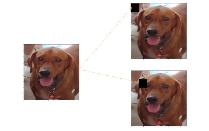
• Select an image and create are occluded copies. The number of copies will depend upon the size of the occlusion. As shown in this depiction

• Get the last convolution layer's output for the Original Image
• Get the same output for all the occluded images and note the average dip across the occluded region.
• The dip will represent the importance(Heatmap) of the region i.e. all the pixels
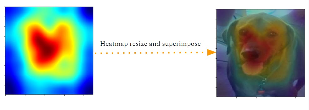
• Resize the heatmap and superimpose on the original image

Note -
^{We have changed the strategy a bit as compared to the original paper. Paper has suggested to do it for the Strongest Filter but this will work equally well and reduce the overhead to find the Strongest filter}

The Code

In the below snippet, we have defined the parameters for image size and patch. Then using a nested loop we have created the Occluded images.

# Defining parameters
size = 224
patch_size = 32
num_images = int((size/patch_size)**2)

import cv2
img = cv2.normalize(img, None, alpha = 0, beta = 255, norm_type = cv2.NORM_MINMAX, dtype = cv2.CV_8UC3)
plt.imshow(img)

# Creating different image occluded at different position
x = np.zeros((num_images, size, size, 3),dtype=int)  #1
x[:] = img  #2

i=j=k=0
while i < size: 
    while j < size:
        x[k,i:i+patch_size,j:j+patch_size,:] = 0.  #3
        j+=patch_size
        k+=1
    i+=patch_size
    j=0

Code-explanation
^{#1 - Blank array to hold all the occluded images. num_images will depend on the patch size, smaller the patch bigger the count
#2 - Filing all the image slots with the original image. Then in the next step, we will put a patch on a different location
#3 - Slicing a portion and occluding it by filling with zero. Loop to move across images and pixels.}

In the below snippet, we have preprocessed the whole image with ResNet pre-process function. Then calculated the dip on the prediction for the Original image and Occluded image

x = preprocess_input(x) 

# Creating a Model to get the prediction for Conv Layer
model_b = keras.Sequential()
model_b.add(base_model)  # base_model is ResNet pre-trained conv block
op = model_b.predict(x) # Output of Occluded Image

img_full = np.expand_dims(img, axis=0).copy()
img_full = preprocess_input(img_full)
img_full_op = model_b.predict(img_full) # Output of all the Original Images

# Calculate the dip and making ignoring the Spikes
act_dip = img_full_op - op
act_max_fm = act_dip.mean(axis=1).mean(axis=1).max(axis=1) #1, #2

heatmap = act_max_fm.reshape(int(size/patch_size),int(size/patch_size)) #3

Code-explanation
^{#1 - act_max_fm is of shape (49, 7, 7 2048). 49 for the Occluded images. 7x7 is the Featuremap size of ResNet last Conv. layer. 2048 is the count of Feature maps. We calculated the mean for each feature map and then the max of the 2048 such outputs.
#2 - So the assumption is that the FM which was most important will have the biggest dip and should come out in max operation.
#3 -act_max_fm is a 1-D array, so we reshaped it to 2-D i.e. 7x7 from (49,)}

In the below snippet, we have simply added the colour map to the heatmap and Superimposed it to the original image using OpenCV functions.

# Normalizing and applying color map to the Heatmap
import cv2
hm = heatmap.copy()    
hm = cv2.normalize(hm, None, alpha = 0, beta = 255, norm_type = cv2.NORM_MINMAX, dtype = cv2.CV_8UC3)
hm = cv2.resize(hm, None, fx=patch_size, fy=patch_size, interpolation = cv2.INTER_CUBIC)
hm = cv2.applyColorMap(hm, cv2.COLORMAP_JET)[:,:,::-1] # Flipped BGR to RGB       

superimposed_img = cv2.addWeighted(img, 0.5, hm, 0.25, 0,)

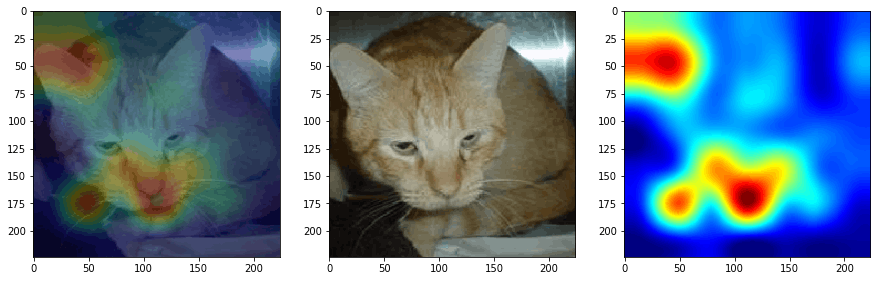
_, ax = plt.subplots(1,3,figsize=(15,5))
ax[0].imshow(superimposed_img, cmap='jet')
ax[1].imshow(img, cmap='jet')
ax[2].imshow(hm, cmap='jet')

Summary and conclusion

While this approach was very intuitive i.e. even if you don't understand the Knitty-gritty of a CNN, you can understand that this should work.

On the down-side,

1. It requires a lot of extra computation in terms of creating and predicting all the images through the Model. To get an estimate for this issue, for an image of size 224x224 and occlusion size of 4x4, we need 3136 images which are equivalent to 313632242248 Bytes ~ 4 GBs of memory
2. Heat map fluctuates a lot based on the size of the patch and the method to pick the dip in Feature maps i.e. Mean, max, etc.

So, we need an approach where we don't have to pass the CNN multiple times. That is where we apply the concept of Class Activation Map Paper

We will learn this technique in the next part of this blog series. Check it Here