Introduction

This is the second post of the Outlier series. We will learn how to catch the Outliers Or Anomalous data points. Don't worry about the terminology, we have covered that in the first part.

In the process, we will develop a high-level understanding of the 4 key algorithms for the purpose and also understand the working of these algorithms. We will also learn to program an Anomaly detector using these algorithms.

We have already Learnt [Check the part-I here ],

• Clarifying the taxonomies around Anomaly detection
• Understanding and applying GaussianMixtureModel

In this post, we will Learn,

• Understanding and applying IsolationForest
• Understanding and applying LocalOutlierFactor
• Using the reconstruction error of PCA

Model - II - Isolation Forest

How it works

In this model, we build a RandomForest of DecisionTrees. Each DecisionTree is built on Random splits and Random Feature selection. If we build a tree following the above approach, an Outlier that is sitting very far from the normal datasets must be split early in the full tree. Definitely, this will not happen for every Tree but it should average out when a decent number of Trees are used in a RandomForest. So, we can simply count the depth required for a point to get isolated. An outlier will have a very small depth. Check the depiction below -

Be mindful of the fact that this distinction is possible only after averaging the split over many DecisionTree. With a single DecisionTree, it can't be guaranteed.

Excerpts from the Scikit-learn documents
^{The IsolationForest ‘isolates’ observations by randomly selecting a feature and then randomly selecting a split value between the maximum and minimum values of the selected feature. Since recursive partitioning can be represented by a tree structure, the number of splitting required to isolate a sample is equivalent to the path length from the root node to the terminating node. This path length averaged over a forest of such random trees, is a measure of normality and our decision function. Random partitioning produces noticeably shorter paths for anomalies. Hence, when a forest of random trees collectively produces shorter path lengths for particular samples, they are highly likely to be anomalies.}

Let's see the Code

By design scikit-learn's IsolationForest is for Outlier detection rather than Novelty detection as it uses a parameter i.e. contamination to identify the Threshold for Outlier and its predict method simply output class i.e. Normal vs Outlier. But we will use it the way we did with GMM.

from sklearn.ensemble import IsolationForest
model = IsolationForest(random_state=0, contamination=0.025).fit(x_train) #1

y_pred = model.predict(x_test_normal)  #2
false_postive = sum(y_pred==-1)

y_pred = model.predict(x_test_outlier)
true_postive = sum(y_pred==-1)

Code-explanation
^{#1 - Kept contamination= 0.025
#2 - Predict function results in +1, -1 for Normal and Outlier respectively}

Result
^{Outliers - All 2203 out of 2203 identified
Normal - 67 out of 2500 incorrectly identified}

Model - III - KNN LocalOutlierFactor

How it works

This model uses a KNN approach to find out the density of data around each data point. If a data point is an Outlier then the density of the data point will be similar to its Neighbour since Outliers points are neighbour to each other. Let's see this depiction -

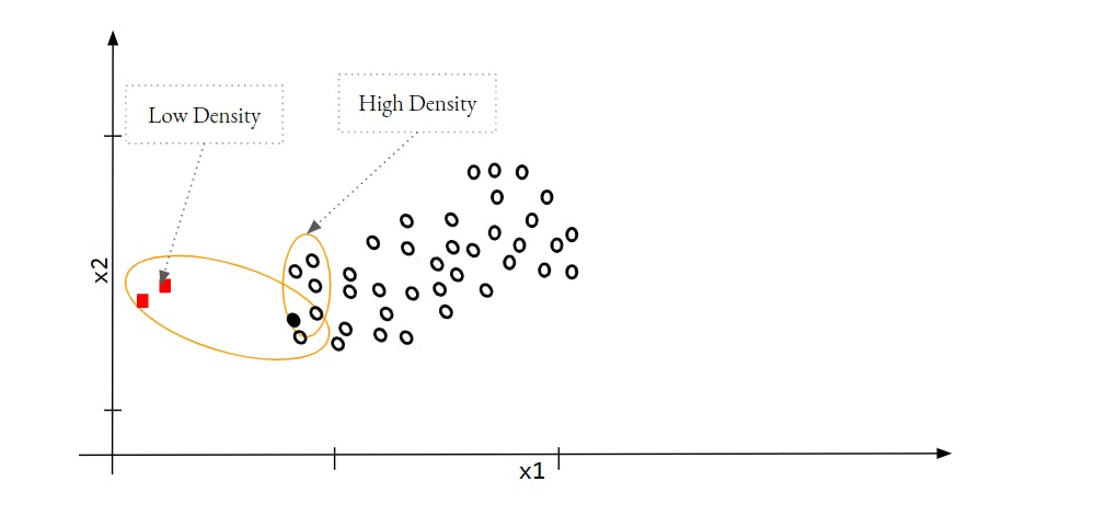
In the image,
^{If we consider one of the Outlier as the first point then its density and the density of its neighbour i.e. the black solid point is quite different. In the case of normal data points, These densities should be similar.}

Excerpts from the Scikit-learn document
^{The anomaly score of each sample is called the Local Outlier Factor. It measures the local deviation of the density of a given sample with respect to its neighbours. It is local in that the anomaly score depends on how isolated the object is with respect to the surrounding neighbourhood. More precisely, the locality is given by k-nearest neighbours, whose distance is used to estimate the local density. By comparing the local density of a sample to the local densities of its neighbours, one can identify samples that have a substantially lower density than their neighbours. These are considered outliers.}

Let's see the Code

from sklearn.neighbors import LocalOutlierFactor

model = LocalOutlierFactor(n_neighbors=10,novelty=True).fit(x_train)

y_pred = model.predict(x_test_normal) 
false_postive = sum(y_pred==-1)

y_pred = model.predict(x_test_outlier)
true_postive = sum(y_pred==-1)

Code-explanation
^{Very similar to the IsolationForest but we have to use the parameter "novelty" to get the +1, -1 output from predict. Also, we have not to tune it for the K but you can try. Lastly, this model is computationally very inefficient}

Result
^{Outliers - All 2203 out of 2203 identified
Normal - 100 out of 2500 incorrectly identified}

Model - IV - PCA's reconstruction error

How it works

In the approach, we use the reconstruction error of PCA. If we reduce the dimension of a dataset using PCA and then try to revert it back to the initial dimension, it will have a reconstruction error for all the points. The dataset has lost the information along the dimension which was removed while reducing the dimension. Since we expect an outler to lie far away from the key principal component[Actually that is the reason it is an Outlier], it will have a high reconstruction error as compared to Inliers. Check the depiction below

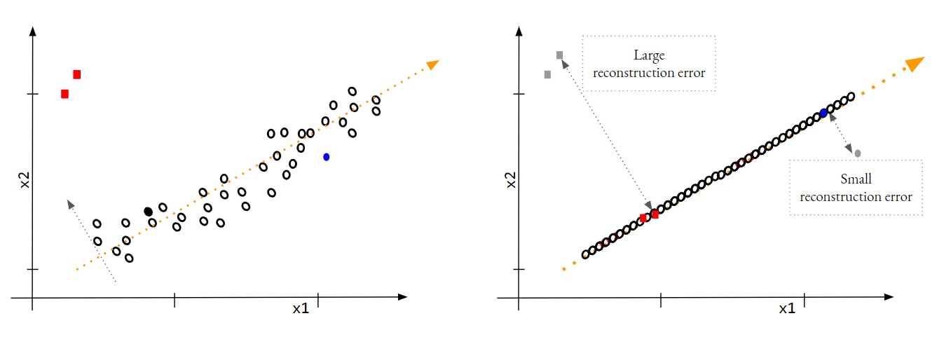
If you observe the Outliers points have larger reconstruction error as compared to the average error of Inliers data points. This is the information that we can utilize to catch the Outliers.

Let's see the Code

We will not do the full coding for this approach but I will put the required steps.

• Reduce the dimension for the data. Will need some tuning here to find out the best n_components.
• Reconstruct the data points. Use scikit-learn PCA's inverse_transform function
• Calculate the error i.e. Cosine similarity, Euclidean distance. Use metrics.pairwise module. It has all the required functions
• Define the Threshold i.e. around 2.5 percentile of errors
• Calculate the error for new data and map the Class based on the Threshold

Conclusions and the way forward

The dataset was relatively easy but appropriate to explain the concept. Adding more data of KDD cup could add other issues i.e. a lot of Categorical features and the post would get diverted. You must try other variants of the available dataset of the KDD cup. Try completing the code for the PCA approach following the mentioned steps. You may also try these concepts on Credit-Card-Fraud dataset available on Kaggle. When the Outlier and Inliers are quite close and it is difficult to find a clear boundary then we must study the False-Positive, False-Negative and try to come up with new Features. Point is that Exploratory Data analysis is always required and we must invest time in it.

Finding the Threshold, we followed a completely unsupervised approach but since we had got the Label for our dataset, we may work in a semi-supervised way to figure out the appropriate Threshold to have a minimum of False-positive and False-Negative.