Introduction

Hello AI Enthusiasts, this is the second part of our series on Natural Language Processing(NLP). You can check the first post [Here]. In the previous post, we used the One-Hot-Encoded data making it similar to Tabular data and used the SVM ML model.
In this post, we will keep the sequence of words intact and use a Recurrent based Neural Network. We will not deep dive into the working of Recurrent based neural Newtowk but put a quick and intuitive summary in the next section. It will help you to move forward throughout this series.
By the end of this post, you will understand the data setup and working of an RNN(Recurrent based Neural Network)

Recurrent based Neural Network

Let's check this depiction similar to a simple Neural Network except for an additional Recurrent weight.

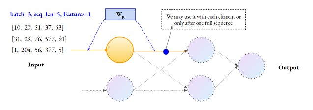
Our data is in the form of a sequence of Words encoded into Integers. Batch has the same meaning as in the case of a simple Neural Network.

• Each sequence element is passed one by one
• The output of each Neuron is looped back via a weight to the input. This facilitates a simple Historical memory. Now the Network has a basic system in place to learn the sequence as a whole rather than each Feature (Word) independently.
• After each Word, the Neuron will output a value. We may pass this output after each word or we may pass it only after the whole sequence(one data point). This decision depends on the use-case. More on it in the next section.
• Since each sequence is passed separately, the length of each data point can be different.
• We have different variants of Recurrent Neural Network. Three of the most common are Simple RNN, LSTM and GRU. Keras has got the implementation of all of these.

This much information is sufficient for us to move forward. In case you want to dive deep into the working of the different implementation, check the book D2L _CH#08,09

Different Input, Output combination

Check the below depiction on the different combination of input type and output type,

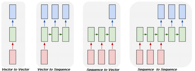
^{Vector is the traditional data points i.e. NxM features based data Or an OHE output
Sequence is the data where datapoints sequence has a meaning e.g. Text, Timeseries data, Speech etc.
_{Image credit - Deep Learning for Computer Vision Fall 2020}}

Let's quickly understand these different combinations,

• Vector to Vector - This is a typical tabular data i.e. Iris data(Vector) and Iris Class(Vector).
• Vector to Sequence - An image captioning system. Image data is a vector.
• Sequence to Vector - Classification(Vector) on IMDB reviews(Sequence ).
• Sequence to Sequence - Language translation i.e. English(Sequence ) to Hindi(Sequence).

^{Let's come back to the blue dot in the first image, we will be interested only in the final output of a full sequence when we are doing the Classification work(case-III) but when we are implementing a translation system(Case-IV), we will need the output after every word. Keep this intuition in mind, we will need it.}

Let's see the code

We are good with the basic theory. Let's code it. Most of the portion will remain same as in the previous post of the Series.

from tensorflow import keras
import numpy as np, seaborn as sns, pandas as pd

num_words=None; maxlen=1000 ; skip_top=20

(x_train, y_train), (x_test, y_test) = keras.datasets.imdb.load_data(num_words=num_words, maxlen=maxlen, skip_top=skip_top)

Code-explanation
^{All other parts of the code is quite trivial and self-explanatory. We don't restrict the word-length and the document counts because Neural Network is an incremental optimization algorithm, unlike the SVM which we used in the previous post. So, it will pretty good with such a volume of data.}

# Dataset to Fixed-lenth by padding #1
clip_length = 250
x_train_ohe = np.zeros((len(x_train), maxlen), dtype='float32')
for i,review in enumerate(x_train):
    j=0
    for word in review:
        if word not in [0,1,2]:
            x_train_ohe[i,j]=word
            j+=1

x_test_ohe = np.zeros((len(x_test), maxlen), dtype='float32')
for i,review in enumerate(x_test):
    j=0
    for word in review:
        if word not in [0,1,2]: #2
            x_test_ohe[i,j]=word
            j+=1

x_train_ohe = x_train_ohe[:,:clip_length]  
x_test_ohe = x_test_ohe[:,:clip_length]

x_train_ohe = x_train_ohe[:,:,np.newaxis] #3
x_test_ohe = x_test_ohe[:,:,np.newaxis]

vocab = int(max(set(x_train_ohe.ravel())))  #4

Code-explanation
^{#1 - Check this image to understand what is done using the two loops. We have initialized a zero-array to standardized the length. Then fill with all the sequences and at the end clipped it to a desired length i.e. clip_length parameter. #2 - [0, 1, 2] are not sentiment word but punctuation words, so skipped it
#3 - Added an axis for the Features. We have only one feature per word.
#4 - Calculated the unique word count. To be used later}

embed_size = 32
model = keras.models.Sequential([
    keras.layers.Embedding(vocab + 1, embed_size, input_shape=[None],mask_zero=True), #1
    keras.layers.GRU(embed_size, return_sequences=True, dropout=0.5), #2
    keras.layers.GRU(embed_size, dropout=0.5),
    keras.layers.Dense(1, activation="sigmoid")
])
model.compile(loss="binary_crossentropy", optimizer="adam", metrics=["accuracy"])

history = model.fit(x_train_ohe,y_train, epochs=2, validation_data=(x_test_ohe,y_test), batch_size=128)#

Code-explanation
^{#1 - We will explain it in next section.
#2 - we have used a GRU recurrent layer. Parameters are self-explanatory
return_sequences -This is the parameter to control the flow of sequence after each word as explained with the blue-dot in the beginning. Setting it True means we have passed the sequence word-by-word. We do this for all recurrent layers before that last one. It means, both the GRU layers will learn in recurrence on each word of a sequence and at the end, it will pass the output to the Dense layer
All other parts of the code is quite trivial and self-explanatory.}

Result
^{Epoch 1/2
195/195 [==============================] - 22s 79ms/step - loss: 0.6104 - accuracy: 0.6331 - val_loss: 0.3225 - val_accuracy: 0.8656
Epoch 2/2
195/195 [==============================] - 13s 66ms/step - loss: 0.2166 - accuracy: 0.9200 - val_loss: 0.3108 - val_accuracy: 0.8700}

Embedding Layer

The first layer we have used in the code snippet was an Embedding layer. This technique has become the backbone of contemporary advancement in the NLP space. We will have a dedicated post on this in the next part of this series.
In simple terms, you may assume this is a Dimensionality reduction technique that tried to represent all the words in N dimensions(32 in our case).
Another benefit that it facilitates is that it converts the sparse OHE encoded data to a continuous space. Neural Network converged easily on a continuous dataset.
Check this post of 10xAI Link to understand the basics of the Embedding Layer.

Conclusion

With the last snippet, we completed this post covering the Recurrent Neural Network. You may try -

• SimpleRNN and LSTM layers of Keras
• Different embedding size
• Different Neurons count

The improvement over the previous model i.e. OHE with SVM is not quite a lot. The primary reason for this is that only a few of the important words are sufficient for Positive/Negative sentiment classification. If you execute the code without a GPU environment, it will take a bit longer. Please use Google Colab for a Free GPU facility.
In the next part of this series, we will dive deep into Word-Embedding and also pre-trained Embeddings.