


Introduction
In this 10xAI's knowledge article, we will understand the Feature Interaction effect in Machine Learning. We will also understand its impact, techniques to find it. In the learning process, we will also understand a very important Feature vs Target plot i.e. Partial Dependent Plot.
Features will be said to have an Interaction effect when the target increased or decreased more than when the two features are present together compared to their individual effect on the target.
$$y = \alpha f1 + \beta f2 + \gamma f1f2 $$
In the above equation, f1 and f2 are two features and f1f2 term is the interaction effect
Interaction Effect can be of multiple types i.e. don't expect it always to be additive. We will not cover too much theoretical detail. You can read more on this in the beautiful book by Max Kuhn and Kjell Johnson [Here]
What is the effect of feature Interaction
Two key effects of Feature Interaction are
- Not all models are able to figure out the effect inherently, so such models will miss this important information
- It affect our interpretation of Feature Importance e.g. in the above case f1,f2 will have higher importance when present together
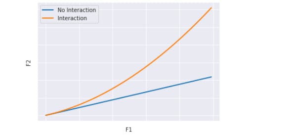
The LinearRegression model will not consider the interaction term by default. We can add such terms by using Polynomial Features. We can observe in the plot below, how the target will move when there is an Interaction effect, and when itis absent.
It's obvious that a LinearRegression will not be able to model the pattern when the effect is present.
A tree-based model is able to capture the Feature Interaction effect inherently. This looks surprising. Try to guess the reason and post your answer in the comment.
Let's see the Code
Let's check a Regression model on California Housing Data, We will follow the following steps.
- Fit a Linear Regression Model on the data set
- Check the coef of each feature to see the Importance
- Create polynomial features and repeat the step but with L1 regularization so that we get rid of not so useful features
- Observe the new Features which are added to feature importance ranking. These will a mix of Interacted-Features and Degree 2 features
# .....Load and pre-process te data #1

# Define Model and fit data

from sklearn.linear_model import SGDRegressor
model_reg = SGDRegressor(eta0=0.001) # eta0=0.001

model_reg.fit(x_train, y_train)

# Check Coeff
coef = pd.DataFrame(model_reg.coef_.reshape(1, -1), columns = x_train.columns) #2
df = coef.T.sort_values(by=[0], ascending=False, key=lambda col: col.abs()) #3
df
Code-explanation
#1 - California housing data is available in Google Colab's sample data folder. You can simply load and pre-process it.
#2,#3 - Get the coeff and sort it. Remember that importance is decided by Magitude not the sign, that's why we passed a function to compare only the absolute value.
Result
latitude >longitude >median_income >population> total_bedrooms >households >total_rooms >housing_median_age
As we can observe, latitude and longitude are the most important features. Followed by median_income. We will not discuss much on feature important as that in itself worth a full post. Now let's repeat the exercise with polynomial features
# Polynomial Features
def poly_feat(x,deg):   #1
    from sklearn.preprocessing import PolynomialFeatures

    poly = PolynomialFeatures(degree = deg)
    x = pd.DataFrame(poly.fit_transform(x), columns=poly.get_feature_names(x.columns))

    return x

d = 2
x_train = poly_feat(x_train, d)  #2

# Very strong L1 Regularization
from sklearn.linear_model import Lasso

model_reg = Lasso(alpha=253, max_iter=5000)  #3
model_reg.fit(x_train, y_train)

# Check Coeff
coef = pd.DataFrame(model_reg.coef_.reshape(1, -1), columns = x_train.columns)
df = coef.T.sort_values(by=[0], ascending=False, key=lambda col: col.abs())
df
Code-explanation
#1 - Function to create polynomial features. It is available in Scikit-Learn.
#2,#3 - Calling the above function and fitting to a LASSO model.
Result
latitude >longitude> total_bedrooms>median_income>population>latitude median_income>total_rooms>longitude median_income>.........
We can observe that the Interacted features of Latitude/Longitude with median_Income has come up in the importance ranking. This hints towards a probable interaction effect between the Features.
This was an indirect technique but intuitive to explain the effect. Now in the next section, let's understand an approach to figure it out
Partial Dependence and its Plot
A partial dependence plot tells us how a Feature impacts the Target assuming all other features as constant. Using this information, we can figure out the Interaction between two features.
Let's understand the general math first.
Let's assume two features F1, F2 contributes to the output as 50, 50 (a fictitious unit). The contribution due to their interaction is 25.
When both the features are used,
total contribution = 125
When only one feature is used
F1, F2 contribution = 50 (because interaction effect will not come into play)
⇒ Difference = 125 - [50(for f1) + 50(for f2) + 0(for Interaction)] = 25
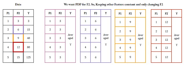
This is a general approach to figure out the interaction effect. This was a basic approach to develop intuition. Let's understand the formal way to do it. There may be some other approaches but we will discuss the approach known as partial dependence plot.We need to do some data Feature twisting/turning before we draw the plot. Here are the steps -
- Replace all the values for a particular feature with a constant value, keep other feature as it is
- Calculate the target and calculate its average for all the samples. This is our first point for one value of
the feature[Check the Image below] - Repeat the above steps for all the different values for the feature
- This will give us the Feature-Target mapping with other feature being constant
We can do the same for two features together. Hence, partial_dependence(F1)+partial_dependence(F2) will be compared with partial_dependence(F1,F2 joint) to figure out the interaction effect.
Let's Code it
We don't need to do it all as Scikit-learn has got a module to do so.
from sklearn.inspection import partial_dependence

features = [1] #latitude
par_1 = partial_dependence(model_reg, x_train, features, method='auto',)
par_1_pred = par_1[0][0]

features = [7]   #median_income
par_7 = partial_dependence(model_reg, x_train, features, method='auto',)
par_7_pred = par_7[0][0]

features = [(1, 7)]  #joint partial_dependence
par_1_7 = partial_dependence(model_reg, x_train, features, method='auto')
joint_pred  = par_1_7[0][0][:,0]
Code-explanation
We have simply used the partial_dependence Class to calculate the same for latitude, median_income and their joint value.
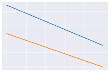
Plot the curve for the sum and joint. In the case of Interaction, the joint plot will move very steeply as compared to the sum of the two features.
plt.plot(par_1_pred+par_7_pred)
plt.plot(joint_pred)
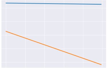
This shows an interaction effect between Latitude and median_income. Let's do the same exercise for latitude and total_rooms.
In this case, both the line have a similar slope. This show an absence of interaction between the two.
The good news is that you don't need to do all this complex exercise. Scikit-Learn provided you with a simple Class to plot the two-way partial_dependence plot.
from sklearn.inspection import plot_partial_dependence

features = [(1, 7)] # latitude and median_income
plot_partial_dependence(model_reg, x_train, features, n_jobs=-1)
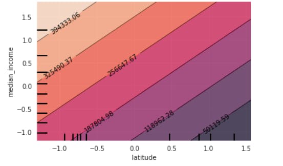
If you read the above plot, with a fixed latitude, the target is moving exponentially(the coloured zone) with median_income. This indicates the presence of Interaction.
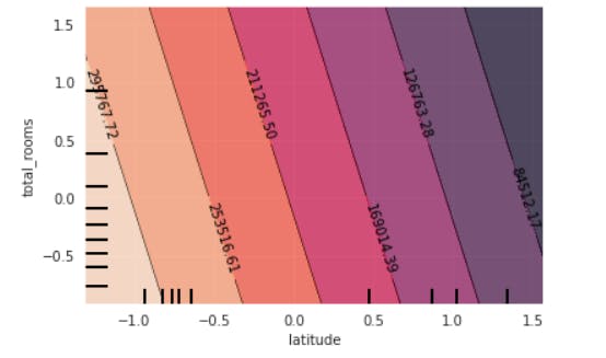
As you would expect, the partial_dependent plot for latitude and total_rooms will not indicate a similar pattern.
Summary and references
You might not need this knowledge always but when the sample and feature volume s not so big and interpretation is a key need. You will need this important concept.
Be mindful that this exercise requires a lot of computation. So this must be considered.
The focus of this post was around the interaction effect, so we exclude the single-feature Vs Target partial_depence plot. You may plot that too using Scikit-learn and understand how a single feature affects the target independent of other features
Read these to dive deep