


Introduction
Correlation among features is one of the most discussed topics in the Machine learning space. While it is very common to find a blog explaining the correlation among Numerical features, it's quite a bit rare to have blogs explaining Correlation among other types of Features.
In this post, we will discuss Correlation among different types of Features and their Python code.
We will learn -
- What are other types of Correlation (other than Pearson's coefficient)
- Intuition to understand the underlying correlation strength
- Python code for individual Correlation method
- Other methods (not discussed in this post)
A quick view of the Dataset
Let's quickly review the dataset that we will use and its respective Features. It's a Life expectancy dataset for different countries.
Due to its nature, it has all different types of Features i.e. Numerical, Categorical, etc. We have created new Features i.e. population_rank so that we have two ordinal Features too.
# Download the data from kaggle
import os, pandas as pd, numpy as np, seaborn as sns, matplotlib.pyplot as plt
os.environ['KAGGLE_USERNAME'] = "10xAI"
os.environ['KAGGLE_KEY'] = "<<Use your Kaggle API Key>>"
import kaggle
!kaggle datasets download kumarajarshi/life-expectancy-who
dataset = pd.read_csv("/content/life-expectancy-who.zip")

# Select 6 columns and 1000 rows
sample = dataset.iloc[:,0:6].sample(1000).reset_index(drop=True)

# This is just to creae another Oridnal Features, so that we have all the combinations of feature types
population = dataset.loc[dataset.Year==2014,['Country','Population']].fillna(0).sort_values(by=['Population']).reset_index(drop=True)
sample['population_rank'] = sample['Country'].apply(lambda x: population[population.Country==x].index.values)
sample['population_rank'] = sample['population_rank'].apply(lambda x: 0 if not x else x[0])

# Fill any NaN
sample.fillna(value=sample.mean(), inplace=True)
sample.iloc[:5,:]
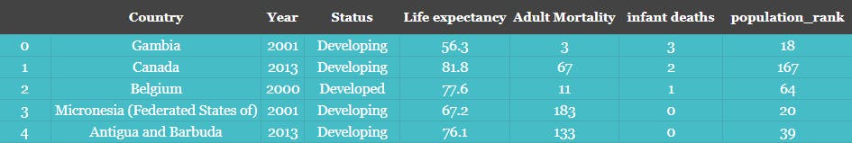 Sample 5 records from the sample DataFrame
Below is mapping for our columns and it's respective type
Year and population_rank as "Ordinal"
Status and Country as "Categorical/Nominal"
Remaining three Features as "Numerical/Continuous"
Method used for different feature pairs
Let's follow a "Top-Down" approach. So we are listing the approaches that we will follow to calculate the correlation between any two types of Features.
In the subsequent section, we will learn the details of all of these and also code the same.
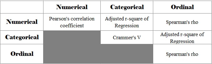
We have only kept the upper Triangle of the table to avoid redundancy because the lower triangle will be a replica of the upper triangle e.g. Numerical-Categorical is the same as Categorical-Numerical
Developing Intuition and understanding the methods
Let's understand each of the used approaches
1. Crammer's V
This method is based on the Chi-square value of two nominal features.
Chi-square value is calculated using the contingency table and the deviation of every value from the expected value. If the expected value is similar to the observed values then we can safely assume a little or no correlation.
Let's understand this by two examples and manual calculation.
| Obesity | No Obesity | Total | |
|---|---|---|---|
| No Gym | 50 (50) | 50 (50) | 100 |
| Gym | 50 (50) | 50 (50) | 100 |
| Total | 100 | 100 | 200 |
We have sample data for 200 cases of individuals and its contingency table for Gym goers and those having Obesity.
A contingency table is simply the cross-tabulated count of different combinations of different Features values. e.g. in the above table, there are 50 data points where Feature#01 has "Gym=Yes" and Features#02 has "Obesity=Yes". This is our observed data
We are trying to answer a simple question " What is the effect of Gym in preventing Obesity"
Let's calculate the expected values using individual totals and grand totals. The expected value is the value for each cell in the contingency table if we assume no relation between the two Features. This can be calculated using a simple formula
Expected value -For "No Gym" - Obesity vs "No Obesity",
There are 100 non-Gym goers. If we assume, no relation between Gym and Obesity, it implies 50% of 100 non-Gym goers will have Obesity and 50% will not have it.
With the above logic, we will have 50 each for Obesity and non-Obesity. Coincidently this value will be the same for all the cells i.e. =50. i.e. values in the parenthesis.
In chi-square logic, we simply calculate the deviation of the observed value from the expected value. i.e.
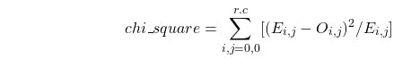
Hence, chi_square = 0, for the above particular scenario. It implies no correlation. It was obvious since the data was created for this purpose.
There is no change in expected value and observed value which implies no correlation between going to Gym and Not being obese.
In other words, had been the aforementioned correlation, the expected value of "Gym, Obese" must be very low, and "Gym, Not Obese" must be high.
Let's see another sample data for the same.
| Obesity | No Obesity | Total | |
|---|---|---|---|
| No Gym | 75 (50) | 25 (50) | 100 |
| Gym | 25 (50) | 75 (50) | 100 |
| Total | 100 | 100 | 200 |
Let's do the calculating again,
Expected values will remain 50 for each case. We will directly calculate the chi_square value.
$$chi-square = (75-50)^2/50 + (25-50)^2/50 + (25-50)^2/50 + (75-50)^2/50$$
= 12.5 + 12.5 + 12.5 + 12.5 = 50 , it shows a good degree of correlation between the two features.
But you might have noticed,
- Since all the terms are positive, having too many unique values of each can increase the value as every new value will add to the total.
- The second issue is that it is difficult to qualify the value i.e. whether the correlation is little or large
With Crammer's V, we fix this issue by standardizing the value w.r.t the sample size and R x C values.
$$Crammer's V = \sqrt({chi_square}/(n * min(r-1, c-1) )$$
n = sample size, r=row count, c= columns count
Crammer's V for the above scenario, = SQRT( 50/(200 x 1) ) = SQRT( 0.25)
= 0.5, which shows a decent correlation
Let's write the Python code for it.
def crammer(s1, s2): #1
    import pandas as pd
    from scipy.stats import chi2_contingency
    n = len(s1)
    r,c = s1.nunique(), s2.nunique()
    matrix = pd.crosstab(s1,s2).values
    chi_sq = chi2_contingency(matrix)
    cramm_V = np.sqrt(chi_sq[0]/(n*min(r-1,c-1)))
    return cramm_V
Code-explanation
#1 - Code is self-explanatory, take the two Features as Pandas Series, calculate the cross-tab matrix and then scipy.stats module calculate the chi_square. Finally, calculate the crammer's V using NumPy functions.
2. Regression Coefficient
We are done with the Nominal to Nominal case. Let's move to the case of Nominal to Continuous and Nominal to the ordinal case. In both these cases, we will use a similar approach.
This approach is quite simple and can be used in most cases. We define one of the variables as an Independent feature and the other as a dependent feature.
Using the two features, we fit a Linear/Logistic Regression model and then calculate the r-square score. Underneath philosophy is that, if the two Feature has little or no correlation, then the Model's score will reflect the same
r-square score of the model is used to get the Strength. Better the r-square score better is the strength. You can read [here] about r-square score.
It's the percentage of variability explained by the model w.r.t to a line passing through the mean. In our case, it will become how one feature can explain the other.
There is a limitation with the r-square score i.e its value increases with every additional feature. So with too many garbage features, it's value will increase and reflect the incorrect relationship.
Although in our case it's just one Feature, still we will use the adjusted r-square score.
It takes into consideration the number of features to balance the addition caused by the increase in r-square score.
Let's proceed to the work -
Categorical - Numerical - Treating Numerical as dependent and converting Categorical to OHE, fit it to a Linear Regression and get the r-square score
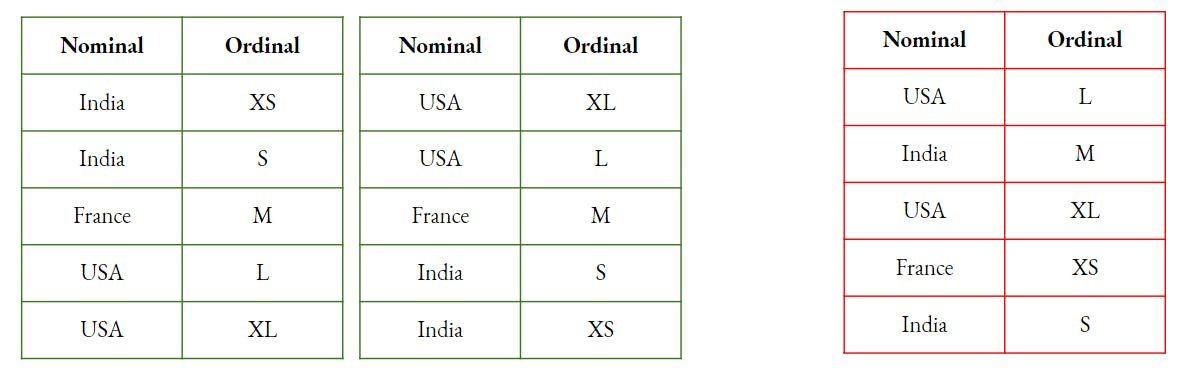
Categorical - Ordinal - In this case, there will be an additional step i.e. to convert the Ordinal feature into a Numerical feature using the Rank. So, basically, we are assuming that if there is a correlation, the prediction will be in a specific direction i.e. either from a smaller rank towards the larger rank or vice-versa.
To create a mental picture for the above explanation, observe the relation in the image below, first two tables show a Correlation while the 3rd table depicts a random relation.
Now, since we are clear with the concept, let's do the coding.
def reg_r2score(s1, s2):
    import pandas as pd
    x, y = (s2,s1) if s2.dtype == object else (s1,s2)  #1
    y=y.rank()
    x = pd.get_dummies(x)
    from sklearn.linear_model import LinearRegression
    reg = LinearRegression().fit(x, y)
    r2score = reg.score(x, y)
    n=len(y)
    k=len(x.columns)
    adj_r_sq = 1 - (1 - r2score)*(n-1)/(n-1-k)
    return adj_r_sq
Code-explanation
#1 - In this line of code, we are simply deciding that the Nominal feature will be x i.e. predictor. Rest all the lines are self-explanatory
3. Spearmen rank-order coefficient
We are done with the case of Nominal to Continuous and Nominal to the Ordinal.
Let's move to the case of Ordinal to Ordinal and Ordinal to Continuous. In both these cases, we will use a similar approach i.e. Spearman’s rank-order coefficient Or Spearmen rho.
Let's understand Spearman’s rank-order coefficient Or Spearmen rho.
It has a simple approach where we rank both the feature among respective values. Then try to measure the difference in respective ranking.
What it means if ranking is similar for both features, we can assume a high correlation. e.g. Academic vs Sports, if the same set of people are top ranker in Academic and the same set of people are either top or bottom ranked, we will assume a very high correlation between the two.
Below is the formula,
$$spearman rho = 1-6\times\Sigma{d_i}^2/n(n^2-1)$$
d is the difference between the respective ranks of the two Features.
The Sum of squares will always increase with additional data points. So the number of data points have been factored in to balanced it.
Let's consider a simple example of Drug Intake(Numerical) and "Rank in Championship"(Ordinal).
| drugs_intake(In grams) | rank in championship | rank of drug intake(since its numerical) | difference (d) |
|---|---|---|---|
| 5 | 2 | 4 | 2 |
| 10 | 3 | 3 | 0 |
| 15 | 4 | 2 | 2 |
| 20 | 1 | 1 | 0 |
$$spearmanrho = 1 - 6 \times (4 + 0 + 4 + 0)/(4\times(16-1)) = 1 - 0.8 = 0.2$$
Lets' do the coding part. In this case, it is very simple i.e. using a module from scipy. Pandas corr() function too can calculate this if passed method='spearman'
def spearman(s1, s2):
    from scipy.stats import spearmanr
    corr, _ = spearmanr(s1,s2) #1
    return corr
Code-explanation
#1 - We are assuming that both the Features are ordinal. Had one been Continuous we would have used the rank function to get the rank as we did in the previous code.
Note - You might have observed that we converted Ordinal into Rank and used regression approach for Ordinal-Nominal and did same for Ordinal-Continuous but calculated spearman's rho. So the whole idea is to measure the movement of one feature w.r.t to the other. If you understand the underlying logic, you can easily have more flexibility.
4. Pearson Correlation
This is the defacto correlation approach. Since most of the time, you deal with Continuous data points and it is used for Continuous features.
We will not explain much of this. You can read about it [Here] .
It give us the linear relationship between the two Features i.e. how one move linearly when the other changes.
For a pair of variables, Pearson’s correlation coefficient is simply the square of the R-square score.
Below is the function to calculate it using scipy. Pandas corr() function too calculates this by Default.
def pearson(s1, s2):
    from scipy.stats import pearsonr
    corr, _ = pearsonr(s1,s2)
    return corr
Conclusion
Just be mindful of the fact that all these techniques are based on different approaches, so you can't compare the output of one with another i.e. 0.5 from Crammer's V might not be the same as 0.5 from the Pearson correlation coefficient.
You may create a function that accepts all the Features and their type and create a consolidated Table or a heatmap. As shown below.
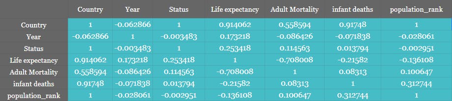
Heatmap
Generating the Heatmap from the Correlation matrix is simple stuff. You can directly call the Heatmap method of Seaborn.
fig, ax = plt.subplots(1, 1, figsize=(10,5))
sns.heatmap(corr_matrix, ax=ax, annot = True)
